Surface Slopes from LiDAR Data (or Fun With Zoning Regulations)
A friend of mine is working with the local zoning board on a rule regulating “steeply” sloped lots in Somerville MA and asked me to do a quick analysis of the number of impacted lots. This project turns out to build on some of the datasets and skills I picked up while building my Parasol Navigation app during my time as an Insight Data Science Fellow.
The core challenge is a neat one: how can we compute the slope of the ground in an urban environment? The key components to my solution were getting my hands on high-resolution elevation observations of the ground surface (without buildings), and figuring out a way to estimate local slopes on a specific length scale from this noisy data.
If you want to run or extend this analysis, all of the code and data you need are hosted at: github.com/keithfma/somerville-slope. As always, feel free to contact me if you would like to discuss further.
Results: Lots of Steep Lots
The zoning rule of interest applies to “all natural slopes exceeding 25% over a horizontal distance of 30 feet”. This sounds like pretty steep, but percent grade has a weird definition: \(\frac{\Delta y}{\Delta x} * 100\). This means that a 100% grade is a slope of 1, or equivalently of 45 degrees, and that grade can be more than 100%. The threshold slope for this rule is actually pretty modest: 7.5 feet of elevation change over a horizontal distance of 30 feet.
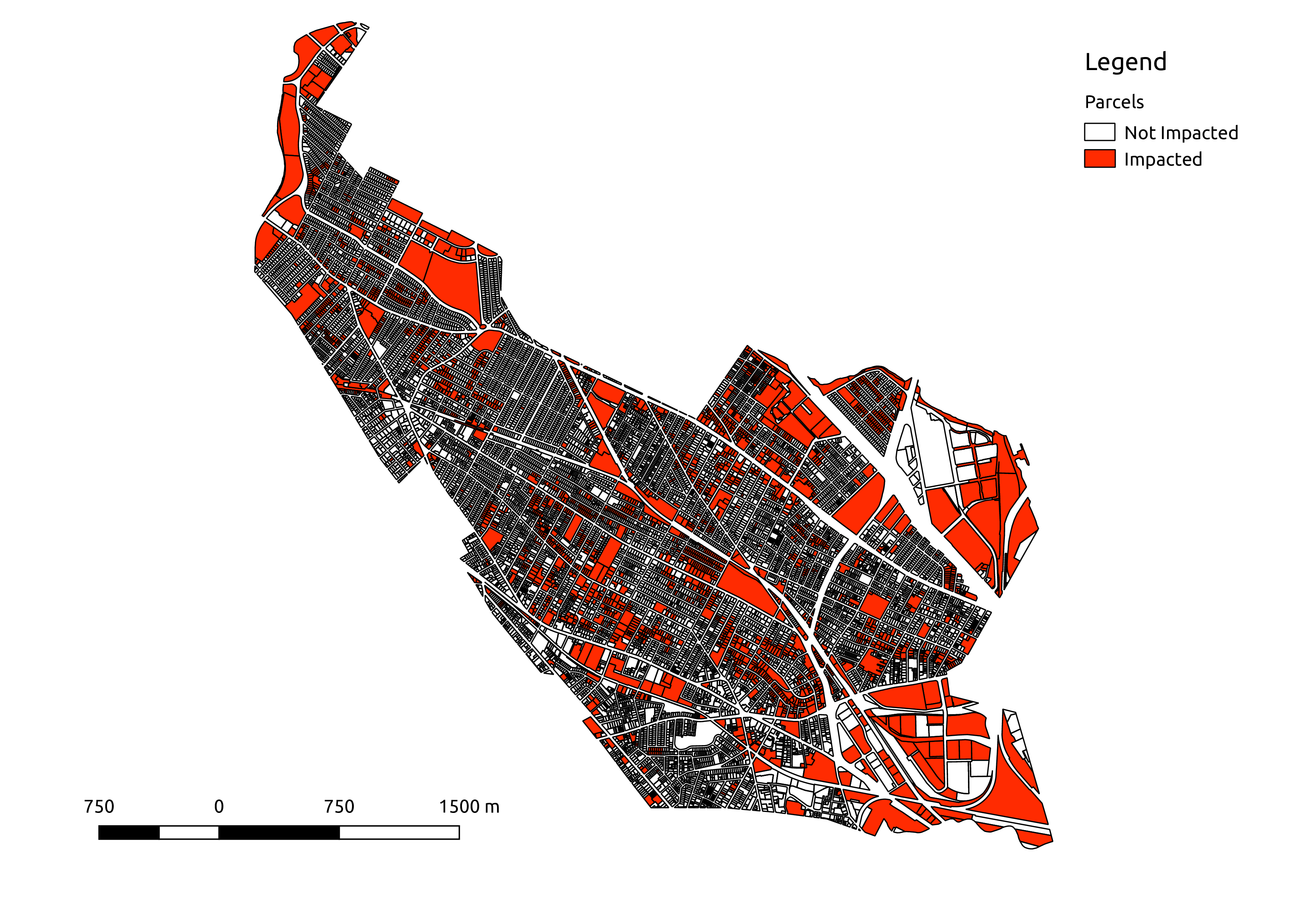
Given this definition, it is not surprising that there are many impacted lots in hilly Somerville MA . I find that 2,370 of 13,354 tax parcels (~18%) contain areas at > 25% grade. The impacted lots are found in clusters around all of the hilly areas in the city.
This result should be of interest to the zoning board, as it was initially assumed that the rule would impact only a few parcels. This is clearly not the case – the rule would in fact come into play throughout the city.
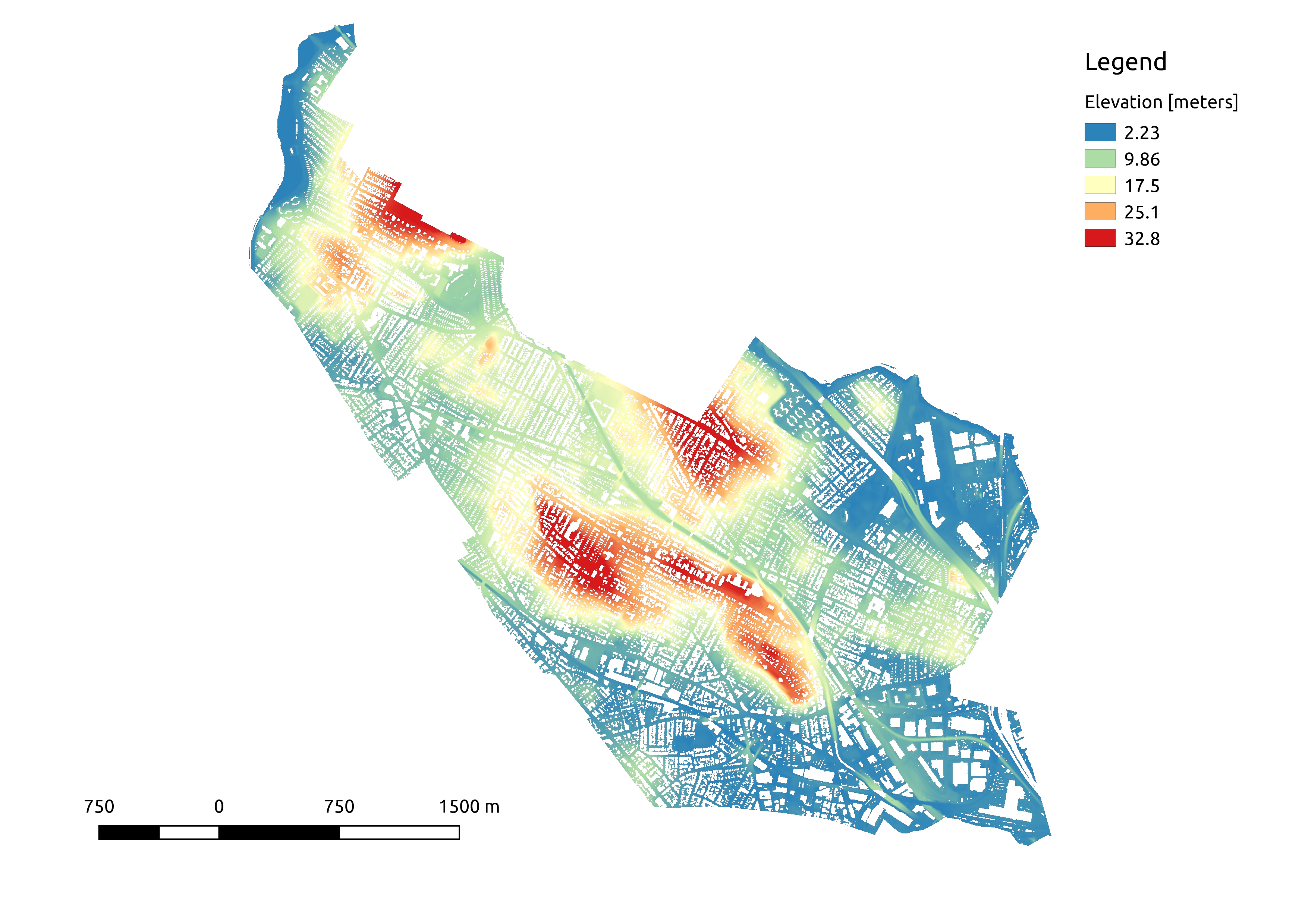
LiDAR Elevation from NOAA
Recent LiDAR surveys conducted in the aftermath of superstorm Sandy provide coverage of the entire city of Somerville. Starting with a shapefiles of MA towns from MassGIS and of the LiDAR tile footprints from NOAA, I gathered up 13 tiles from the NOAA server. Each tile has an average of 3.8 observations per square meter. Nice!
One critical prerequisite for the ground slope analysis to work is that estimated slopes must exclude buildings and trees. Happily, LiDAR contains some extra information that helps in labeling and removing these above-ground features (e.g. multiple returns from tree canopy and ground). Even more happily, this LiDAR dataset classifies for all points as “default”, “ground”, “water”, etc,, meaning that I can simply filter by the label to get the ground-return-only dataset I need.
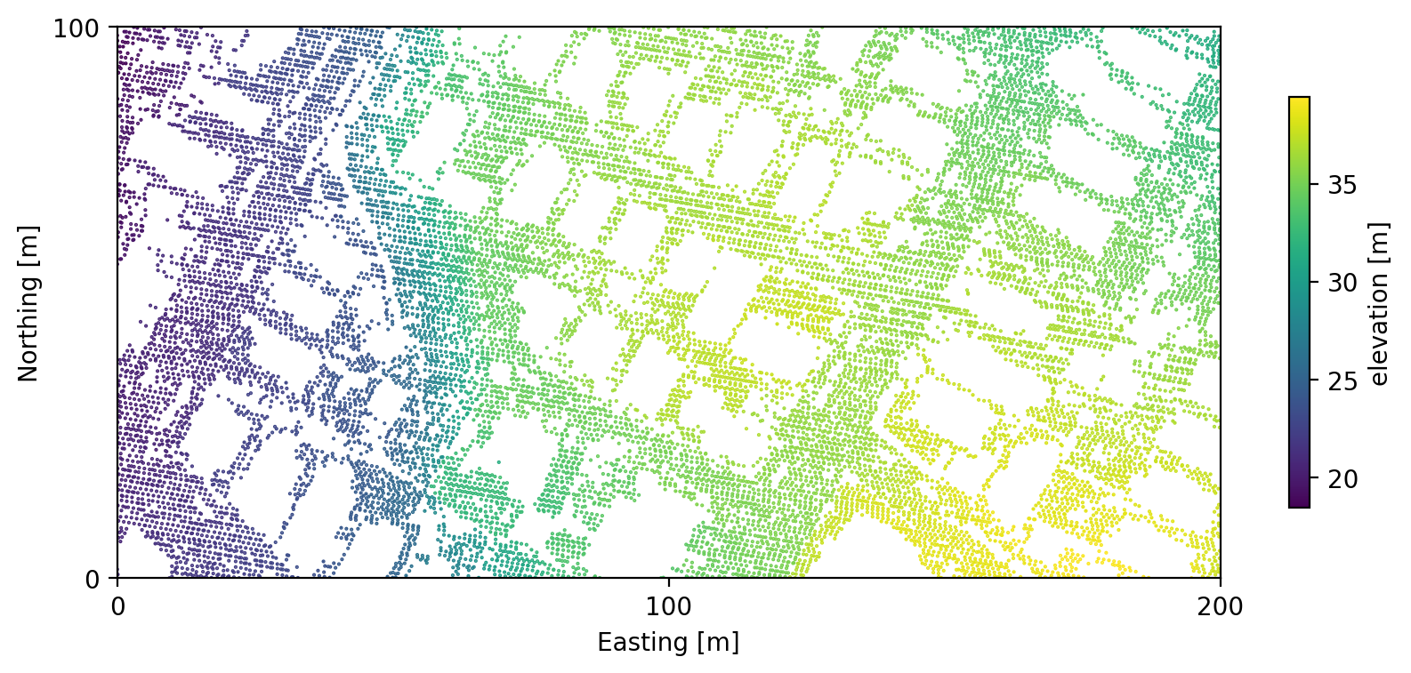
In total, this ground-only dataset contains ~36 million elevation observations. There are “holes” wherever buildings were removed from the dataset, but we do have observations from the ground below the tree canopy.
Analysis: 25,781,323 Least Squares Fits
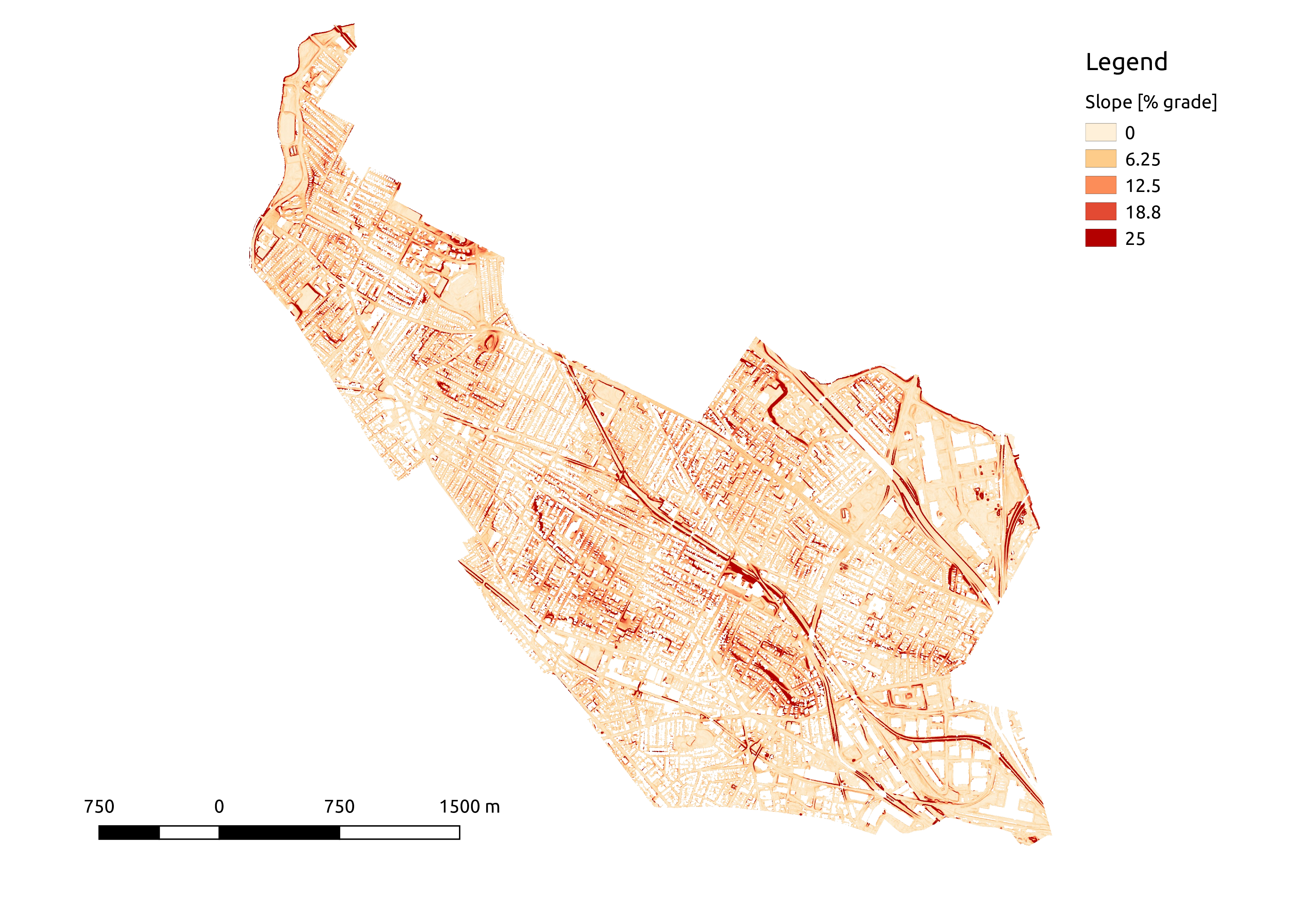
With the elevation data in hand, the next step is to compute local slopes throughout the city. The trick here is that the zoning regulation applies to slopes over a 30-foot length scale. This means that the usual approach of gridding the elevations and using finite differences to approximate the local gradient is a no-go – this would not give the correct lengthscale.
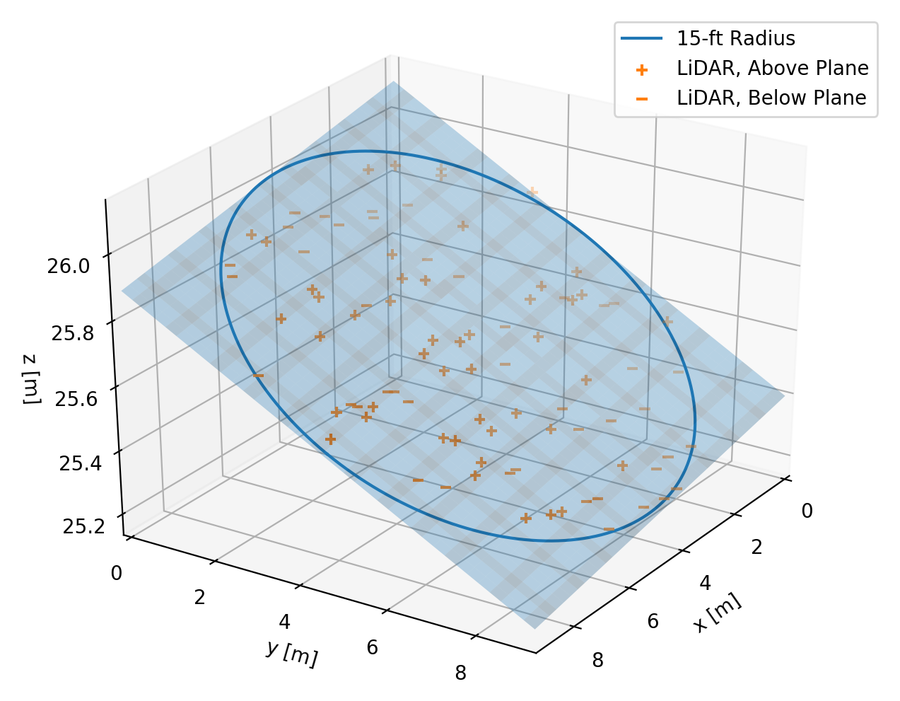
Instead, I decided to estimate the “30-foot slopes” for each point using the best-fit plane to the points within a 15-foot radius. This approach has the advantage that it includes all of the elevation information in the specified area around a point, and simultaneously estimates elevation and slope magnitude and direction.
To dig in just a little, each planar fit finds a plane defined as \(z = ax + by +c\), with the free parameters \(a, b, c\) determined by a standard least squares minimization. Given this equation, the estimate for elevation at a point \((x^\prime, y^\prime)\) is simply \(z^\prime = a x^\prime + b y^\prime +c\). The local slope has components \(\frac{\partial z}{\partial x} = a\) and \(\frac{\partial z}{\partial y} = b\), with magnitude \(\sqrt{a^2 + b^2}\) and direction \(\arctan \left( \frac{b}{a} \right)\).
The calculation is fairly laborious. I created a regular grid with 1 meter spacing over the whole city and a binary mask indicating which points are inside the city limits. Then for each point in this grid, I extracted the LiDAR observations within 15 feet. To make this extraction feasible, I used a KDTree to speed up the spatial lookup (cKDTree is your friend!). Then I solved for the best-fit plane using least squares using numpy.linalg.lstsq to handle all the possible numerical pitfalls for me.
One thing I was worried about in this analysis was the possibility of errors in the original data classification. If there were any points labeled as “ground” that were in fact the edge of some tall building, then I might end up computing erroneously high slopes at the edge of buildings. This would be a serious flaw, given that this is an urban environment and high slopes are the key result I was looking for. To mitigate this risk, I only computed slopes around points whose local 30-foot neighborhood was well populated – with at least 75% of the number of observations expected for an area with no data gaps. This decision eroded slightly the area where I could compute slopes, but in return increased my confidence in the results. This potential issue is not readily apparent in the results, which suggests the procedure worked as expected.
From Slope to Impacted Parcels
The last step was to count the parcels in the city that would be impacted by the zoning regulation. Using a shapefile of the Somerville tax parcels provided by MassGIS, I summed the area with above-threshold (>25%) slope in each parcel. To be conservative in my count, I set an (arbitrary) cutoff of 5 m2 above-threshold slope. Parcels with more than 5 m2 of above-threshold slope were labeled as “impacted”, and all others were labeled as “not impacted”.